So imagine that you've got a bunch of time series representing the same type of obervations, like retail daily sales, hearbeats of joggers or some obscure sensors. There is a big benefit for applying clustering either during data discovery or for modeling the dataset itself, this benefit is mainly linked to the understading of existing similarities between some fractions of the dataset, like gathering together retail points-of-sale that are booming during summer vs the ones booming during chirsmass time, or looking for the right explanation for why 1000 joggers are considered as part of the same group, is there any health issue common to them or is it related to living at high altitudes for example. You've guessed it, there is a lot of positive outputs that can emerge from clustering time series hence the importance of doing it right by avoiding some pitfalls that can make this ineffective or absolutely erroneous.

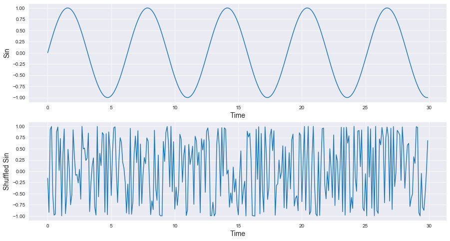
Before going any further, let us take a couple of seconds to ask a fundamental question: What makes time series so special compared to other types of datasets ? Mainly two things, the first one is the "series" part which means each observation is linked to a sequence, a frequency of some sort, a beat, a pulse or something like that. The second thing, represented on the "time" and "chronology" part, is the order of observations, changing the order will be considered as generating a totally different time series. In the following graph, shuffling the \(sin\) signal will produce something other than a \(sin\) even if the dataset is similar (without considering the order of course) because the chronological position for each observation is very important to define our time series.

Something else to be mentioned, a time series is in general defined in a high dimension space. If you happen to record the daily sales of an ice-cream shop during one year, that's a dimension with a cardinality equal to 365, so just imagine if we're having a decade worth of data.

The Curse of Dimensionality

A word or two about distances

When we're speaking about distances, we tend to think right away about the Euclidean distance. Just a quick reminder, the Euclidean distance is defined in an Enclidean Space as

Where \(a\) and \(b\) are two points in space with their respective space coordinates \((x_{a1}, x_{a2}, ..., x_{an})\) and \((x_{b1}, x_{b2}, ..., x_{bn})\) and \(n\) is a strictly positive integer meaning \(n \in \mathbb{N}^*\).

The truth is that the concept of distance is a much more abstract and general one, the Euclidean distance is just one out of many existing distances. We can call a distance anything that fulfill some set of mathematical conditions: If we consider the function \(d\) operating in a set \(E\), with \(d: E\times E\rightarrow \mathbb{R^+}\), \(d\) is called a distance if it satisfies the following conditions :

• Symmetry : \(\forall (a, b) \in E^2,\ d(a, b)=d(b, a)\)
• Coincidence : \(\forall (a, b) \in E^2,\ d(a, b)=0 \Leftrightarrow a=b\)
• Triangle Inequality : \(\forall (a, b, c) \in E^3,\ d(a, c)\leq d(a,b)+d(b,c)\)

So if you happen to create a function that meets this three constraints, congratulations you've created a distance metric!

But why am I talking about all this? How this is relevant to what I'm trying to say ? In fact my main point here is that the Euclidean distance, that we're using instinctively, is not the only existing distance and there is a bunch of other ones like the Manhattan distance, the Cosine distance, the Chebyshev distance, the Minkowski distance just to name a few. And clustering algorithms are strongly based on distance measures, similar points in space means they happen to be close to each others, so changing the distance metric can change to a great extent the behavior of our clustering algorithm. In fact, this applies to a big chunk of machine learning concepts.

High dimension & the curse!

Until now, everything is good and we're happy with our distance metrics. The big question to ask here is, does distance behave similarly in high dimensions ? Can we trust some distance measures to discriminate, which means knowing similarities and non-similarities of the population we're having on our dataset, in high dimension spaces ?

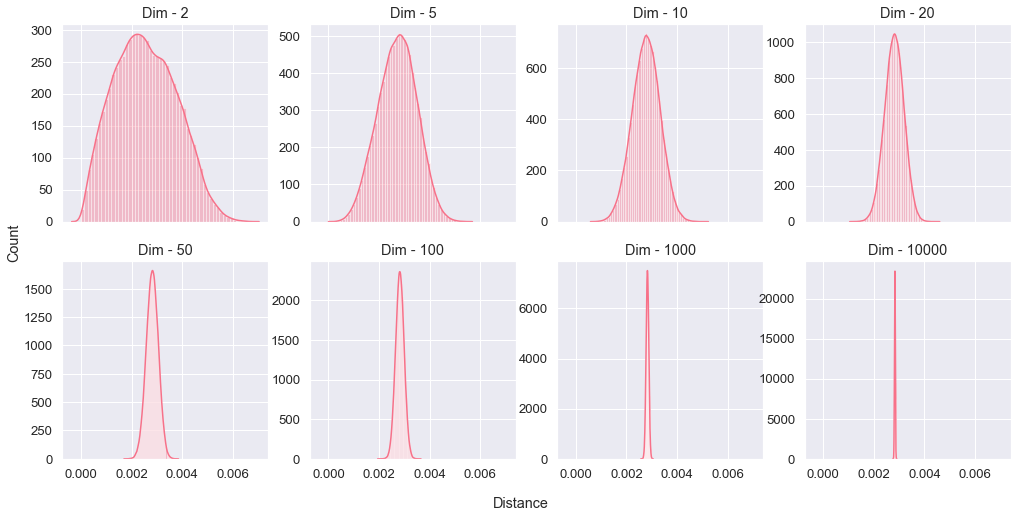
I won't answer right away, but instead I will make a simple experiment. Let's generate 500 random points, uniformly distributed, and then compute the Euclidean distances between all possible pairs (124,750 pairs), then we will plot the distribution of those distances. We will do that by increasing the dimension of our space to see what will happen exactly at high dimensions.

You can test this by yourself by using the following code :

import numpy as np
import scipy as sc
import itertools
import seaborn as sns
import matplotlib.pyplot as plt
from sklearn.preprocessing import normalize
sns.set_style("darkgrid")


num_points = 500
dims = [2, 5, 10, 20, 50, 100, 1000, 10000]
fig, axes = plt.subplots(2, 4, figsize=(17, 8), sharex=True)

for ind, dim in enumerate(dims):
    plot_line = ind // 4
    plot_column = ind % 4
    ax = axes[plot_line, plot_column]
    pairs = itertools.combinations(list(range(num_points)), 2)
    points = np.random.rand(dim, num_points)
    distances = np.zeros(int(sc.special.comb(num_points, 2)))

    pair_ind = 0
    for pair in pairs:
        p1 = points[:, pair[0]]
        p2 = points[:, pair[1]]
        distances[pair_ind] = sc.spatial.distance.euclidean(p1, p2)
        pair_ind += 1

    ax.set_title("Dim - {:d}".format(dim))
    distances = normalize(distances[:,np.newaxis], axis=0)
    sns.distplot(distances, norm_hist=True, ax=ax);

fig.text(0.5, 0.04, 'Distance', ha='center')
fig.text(0.08, 0.5, 'Count', va='center', rotation='vertical');

We observe that at high dimensions there is a decrease of distance variance, with the extrême case of 10,000 dimensions where pairwise distances converge to a very narrow value, it's like all points in space are in a Mexican standoff with no real winner. The fact that we loose the variance of pairwise distances means we can't discriminate the population or find any significant similarities therefore the effort of clustering is doomed to failure.

In the context of clustering time series, a lot of people tend to use the most classical clustering algorithm namely, the K-Means clustering. In its most classical form, it is based on euclidian distance and applying it to time series, like daily sales of ice-cream shops during a decade, is equivalent to use euclidean metric in high dimension which will definitely lead to the curse of dimensionality.

What shall we do then ?

So now that I've given you the bad news, don't think you're hopeless...I will share with you two main strategies to counter the effect of the curse of dimensionality when clustering time series.

Reducing the space by features extraction!

If you want to maintain the way you cluster your time series with no fancy techniques, the best approach is to reduce the space on which your time series are defined. In fact by "reducing" I mean shifting your time series to a complete different space by computing some relevant features observed on your time series like trends, means, maximum values on certain days or entropy for example (here's a list of a non-exhaustive relevant features to be computed). So if we imagine that you'll need just 10 features to describe your time series, depending on your context of course, it will always be definitely better than daily values during a decade (that's around 3,650 features).

There is a very useful library you can use for computing those features called TSFRESH.

Changing how we measure similarities

The second strategy is to completely change the metric, as we've seen it before there is many existing distance metrics and what we need on our case is to pick the metric that will manage to reduce the effect and unfortunately this is not a safe bet.

That's been said, the best measure to use is Dynamic Time Warping (or DTW), even if it's not, mathematically speaking, a distance metric. DTW is an algorithm that measures similarities between two time series, we can use it as a measure for a K-Means clustering and it is, in our context, immune to the curse of dimensionality because at its core the algorithm operates in a two dimensional space.

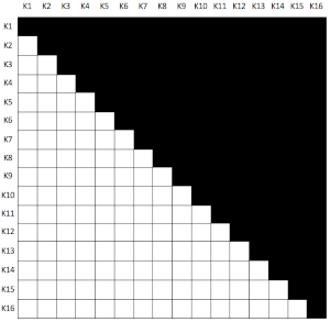
DTW can be a good solution to counter the curse, but it has two major problems when dealing with a dataset with too many time series. The first issue is the need to compute pairwise distances for all existing time series, which is equivalent to create an upper triangular matrix (we consider symmetrical DTW) with an all zero diagonal (a DTW of a time series to itself is zero). For that, we need to compute \(\frac{m^2-m}{2}\) DTWs (where \(m\) is the number of time series we have), so for 1,000 time series we have to compute 499,500 DTW values. The following graph represents the DTW distance matrix shape for 16 time series.

The second issue is the algorithmic performance : the DTW algorithm is a \(O(n^2)\), so for the 1,000 time series computing DTW 499,500 times can take forever!

I wish you'll remember this article when dealing with clustering time series, and I hope it gave you a better understanding about the impact of the curse of dimensionality.

That's all folks! Don't hesitate to follow me on Twitter!